chebyshev#

The chebyshev module is a collection of functions for setting up and using Chebyshev expansions, which can be used for very high accuracy interpolation on smooth problems and for numerical solutions to boundary value problems and PDEs. Since you’re reading this, I assume you already know how awesome Chebyshev expansions are! For the right problems, they have exponential, or “infinite order,” convergence!

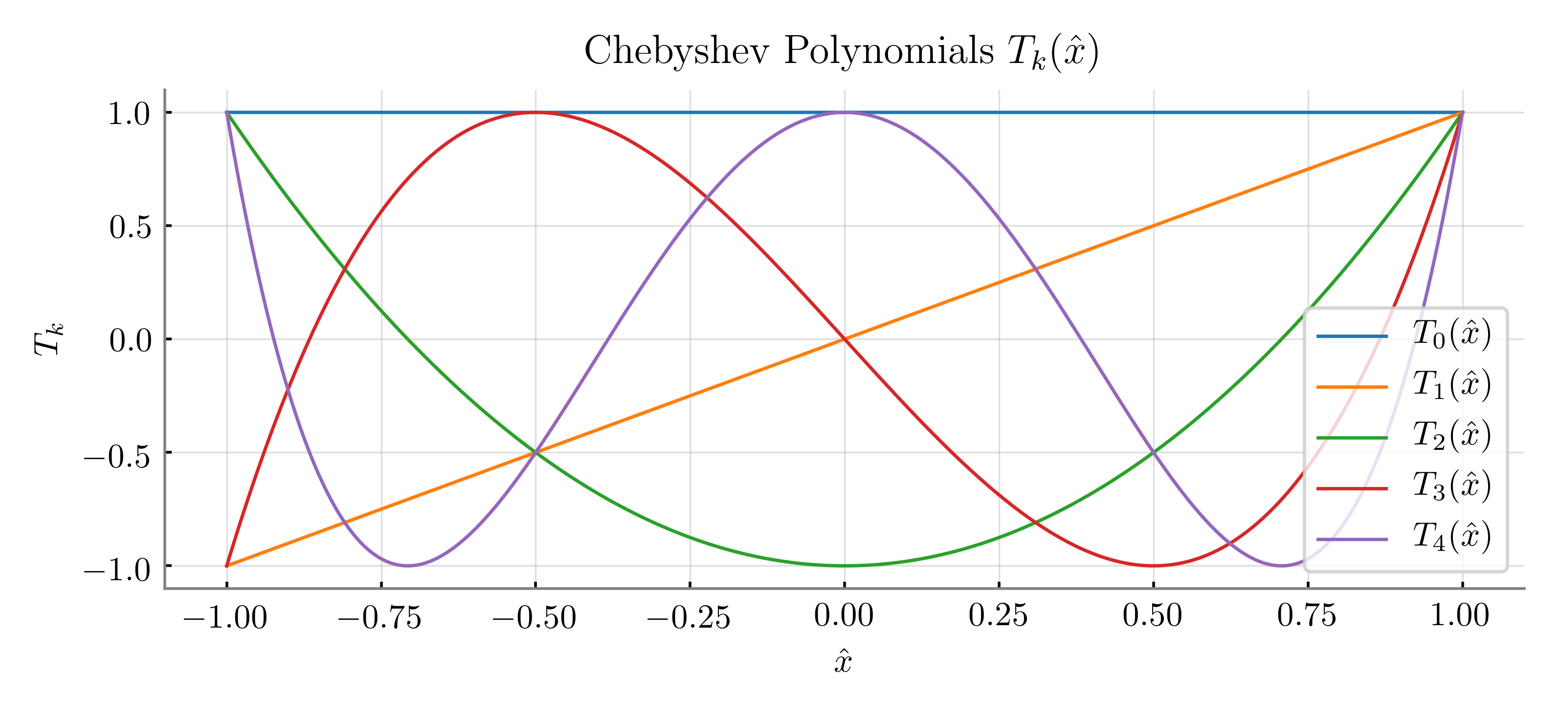
Anyway, Chebyshev polynomials (of the first kind) can be defined and evaluated in a number of ways. Here they are defined by

\[T_k(\hat{x}) = \cos(k \arccos(\hat{x})) \qquad \hat{x} \in [-1,1] \, ,\]

where \(k\) is the degree of the polynomial and \(\hat{x}\). The polynomials are orthogonal with respect to the weighted inner product

\[\left< f(x),g(x) \right> = \int_{-1}^1 f(x) g(x) \frac{1}{\sqrt{1 - x^2}} dx \, .\]

Through a quick transformation, the polynomials can be mapped from \([-1,1]\) to some other interval \([x_a,x_b]\) using

\[x(\hat{x}) = \frac{\hat{x} + 1}{2} (x_b - x_a) + x_a \qquad x \in [x_a,x_b]\]

and back again by

\[\hat{x}(x) = 2 \frac{x - x_a}{x_b - x_a} - 1 \qquad \hat{x} \in [-1,1].\]

It’s often convenient to use a third coordinate, \(\theta\), because of the trigonometric definition of the polynomials. For \(\theta = \cos(\hat{x})\), the Chebyshev polynomials are

\[T_k(\cos(\hat{x})) = T_k(\theta) = \cos(k\theta) ,\]

simply cosines, where \(\theta\) is in the interval \([\pi,0]\). Using \(\theta\) coordinates in addition to the \(\hat{x}\) and \(x\) coordinates simplifies derivatives of the polynomials and enables the use of discrete cosine transformations to obtain expansion coefficients, as implemeneted in the cheby_dct function.

The first couple derivatives of the polynomials can be evaluated with respect to \(\theta\) by using the chain rule to convert to \(\hat{x}\) coordinates. Derivatives then must be scaled to \([x_a,x_b]\) by dividing by \(((x_b - x_a)/2)^p\), where \(p\) is the order of the derivative.

In addition to functions for evaluating the Chebyshev polynomials and their derivatives, some higher level functions are provided by this module.

cheby_bvp_setup creates the grid and matrix used to solve boundary value problems in 1D, capable of handing boundary conditions of arbitrary derivative order and 1st or 2nd internal derivatives.
cheby_coef_setup also creates a grid and matrix, but only to solve for the expansion coefficients, without derivatives. This is just a transform from some set of points to a set of Chebyshev polynomials. It allows for the use of a first derivative on one of the boundaries and for extra points in the grid.
cheby_dct_setup creates a grid for generating chebyshev expansions using the discrete cosine transform (DCT). It does not allow for derivatives or extra points, however. The underlying function for performing a discrete chebyshev transform is cheby_dct and the inverting function is cheby_idct.

Tons of information on these and other methods can be found in these references:

Boyd, John P. Chebyshev and Fourier spectral methods. Courier Corporation, 2001.
Fornberg, Bengt. A practical guide to pseudospectral methods. Vol. 1. Cambridge university press, 1998.
Canuto, Claudio, et al. Spectral methods. Springer-Verlag, Berlin, 2006.

orthopoly.chebyshev.insert_points(xhat, theta, x, xextra, xa, xb)#

Puts some extra points into the cheby grid, ignoring duplicates and keeping things correctly sorted

Parameters:

xhat (array) – grid points on \([-1,1]\)
theta (array) – grid points on \([\pi,0]\)
x (array) – grid points on \([x_a,x_b]\)
xextra (array) – the x points to insert
xa (float) – left boundary
xb (float) – right boundary

Returns:

tuple containing

grid points on \([-1,1]\) with points inserted
grid points on \([\pi,0]\) with points inserted
grid points on \([x_a,x_b]\) with points inserted

orthopoly.chebyshev.cheby_grid(xa, xb, n)#

Computes the chebyshev “extreme points” for use with all the functions in this module

The grid points are in \([-1,1]\) and they are

\[\hat{x}_i = \cos\left(\frac{\pi j}{n-1}\right) \qquad j = n-1,...,0 \, .\]

These points are returned with their counterparts in \(\theta\) and \(x\) coordinates.

Parameters:

xa (float) – value of left (lower) domain boundary
xb (float) – value of right (higher) domain boundary
n (int) – number of points to use in the domain (including boundary points)

Returns:

tuple containing

array of collocation points (\(\hat{x}\) points) in \([-1,1]\)
array of theta values, \(\arccos(\hat{x})\), in \([0,\pi]\)
array collocation points in \([x_a,x_b]\)

orthopoly.chebyshev.cheby(x, k, xa=-1, xb=1)#: Evaluates the \(k^{\textrm{th}}\) chebyshev polynomial in \([x_a,x_b]\) at \(x\)

orthopoly.chebyshev.cheby_hat(xhat, k)#: Evaluates the \(k^{\textrm{th}}\) chebyshev polynomial in \([-1,1]\)

orthopoly.chebyshev.cheby_hat_ext(xhat, k)#

Evaluates a chebyshev polynomial in \(\hat{x}\) space, but potentially outside of \([-1,1]\)

Parameters:

xhat (float/array) – argument
k (int) – polynomial degree

Returns:

\(T_k(\hat{x})\)

orthopoly.chebyshev.dcheby_t(t, k)#: Evaluates the first derivative of the \(k^{\textrm{th}}\) order chebyshev polynomial at theta values

orthopoly.chebyshev.ddcheby_t(t, k)#: Evaluates the second derivative of the \(k^{\textrm{th}}\) order chebyshev polynomial at theta values

orthopoly.chebyshev.dpcheby_boundary(sign, k, p)#

Evaluates the \(p^{\textrm{th}}\) derivative of the \(k^{\textrm{th}}\) order chebyshev polynomial at -1 or 1

Parameters:

sign (int) – -1 or 1
k (int) – polynomial degree
p (int) – derivative order

Returns:

\(d T_k(\pm 1) / dx\)

orthopoly.chebyshev.cheby_sum(x, a, xa, xb)#: Evaluates a chebyshev expansion in \([x_a,x_b]\) with coefficient array \(a_i\) by direct summation of the polynomials

orthopoly.chebyshev.dcheby_t_sum(t, a)#: Evaluates the first derivative of the cheby expansion at \(\theta\) values

orthopoly.chebyshev.cheby_hat_sum(xhat, a)#: Evaluates a chebyshev series in \([-1,1]\) with coefficient array \(a_i\) by direct summation of the polynomials

orthopoly.chebyshev.cheby_hat_ext_sum(xhat, a)#

Evaluates chebyshev expansion anywhere, including outside \([-1,1]\)

Parameters:

xhat (float/array) – argument
a (array) – expansion coefficients \(a_i\)

Returns:

evaluated expansion

orthopoly.chebyshev.dcheby_coef(a)#

Computes the coefficents of the derivative of a Chebyshev expansion using a recurrence relation. Higher order differentiation (using this function repeatedly on the same original coefficents) is mildly ill-conditioned. See these references for more info:

Boyd, John P. Chebyshev and Fourier spectral methods. Courier Corporation, 2001.
Press, William H., et al. Numerical Recipes: The Art of Scientific Computing. 3rd ed., Cambridge University Press, 2007.

Parameters:: a (array) – expansion coefficients \(a_i\)
Returns:: expansion coefficients of the input expansion’s derivative

orthopoly.chebyshev.cheby_hat_recur_sum(xhat, a)#

Evaluates a Chebyshev expansion using a recurrence relationship. This is helpful for things like root finding near the boundaries of the domain because, if the terms are evaluated with \(\arccos\), they are not defined outside the domain. Any tiny departure outside the boundaries triggers a NaN. This recurrence is widely cited, but of course, See

Boyd, John P. Chebyshev and Fourier spectral methods. Courier Corporation, 2001.

Parameters:

xhat (float/array) – argument
a (array) – expansion coefficients \(a_i\)

Returns:

evaluated expansion

orthopoly.chebyshev.dcheby_hat_recur_sum(xhat, a)#

Computes the derivative of a Chebyshev expansion in \([-1,1]\) using a recurrence relation, avoiding division by zero at the boundaries when using dcheby_t. This is the same procedure as in dcheby_coef, but using the derivative coefficients to evaluate the derivative as the recurrence proceeds instead of just storing and returning them.

Parameters:

xhat (float/array) – argument
a (array) – expansion coefficients \(a_i\)

Returns:

evaluated expansion

orthopoly.chebyshev.cheby_dct(y)#

Finds Chebyshev expansion coefficients \(a_k\) using a discrete cosine transform (DCT). For high order expansions, this should be much faster than computing coefficients by solving a linear system.

The input vector is assumed to contain the values for points lying on a chebyshev grid. The Chebyshev expansion is assumed to have the form

\[\sum_{k=0}^{n-1} a_k \cos(k \arccos(\hat{x})) \qquad \hat{x} \in [-1,1]\]

However, because the Type I DCT in scipy.fftpack has a slightly different convention, some small modifications are made to the results of scipy.fftpack.dct to achieve coefficents appropriate for the expansion above.

Parameters:: y (array) – values of points on a chebyshev grid, in the proper order
Returns:: array of Chebyshev coefficients \(a_k\)

orthopoly.chebyshev.cheby_idct(a)#

Evaluates a chebyshev series using the inverse discrete cosine transform. For high order expansions, this should be much faster than direct summation of the polynomials.

The input vector is assumed to contain the values for points lying on a chebyshev grid. The Chebyshev expansion is assumed to have the form

\[\sum_{k=0}^{n-1} a_k \cos(k \arccos(\hat{x})) \qquad \hat{x} \in [-1,1]\]

Because of varying conventions, this function should only be used with chebyshev expansion coefficients computed with the functions in this package (cheby_coef_setup and cheby_dct). The Type I IDCT from scipy.fftpack is used (with minor modifications).

Parameters:: a (array) – chebyshev expansion coefficients \(a_k\)
Returns:: array of evaluated expansion values at chebyshev grid points

orthopoly.chebyshev.cheby_bvp_setup(xa, xb, n, aderiv, ideriv, bderiv, xextra=None)#

Set up the grid and matrices for a Chebyshev spectral solver for boundary value problems in 1 cartesian dimension

Parameters:

xa (float) – value of left (lower) domain boundary
xb (float) – value of right (higher) domain boundary
n (int) – number of points to use in the domain (including boundaries)
aderiv (int) – order of derivative for left boundary condition (can be 0)
ideriv (int) – order of derivative for internal nodes (must be 1 or 2)
bderiv (int) – order of derivative for right boundary condition (can be 0)
xextra – extra points within the domain to include as collocation points

Returns:

tuple containing

collocation points in \([-1,1]\)
theta values, \(\arccos(\hat{x})\), in \([0,\pi]\)
collocation points in \([x_a,x_b]\)
matrix to solve for the expansion coefficients

orthopoly.chebyshev.cheby_coef_setup(xa, xb, n, da=False, db=False, xextra=None)#

Constructs the grid and matrix for finding the coefficients of the chebyshev expansion on \([x_a,x_b]\) with \(n\) points

Parameters:

xa (float) – value of left (lower) domain boundary
xb (float) – value of right (higher) domain boundary
n (int) – number of points to use in the domain (including boundaries)
da (bool) – use the first deriv at the left/low boundary as the boundary condition
da – use the first deriv at the right/high boundary as the boundary condition
xextra (array) – extra points within the domain to include as collocation points

Returns:

tuple containing

collocation points in \([-1,1]\)
theta values, \(\arccos(\hat{x})\), in \([0,\pi]\)
collocation points in \([x_a,x_b]\)
matrix to solve for the expansion coefficients
scale factor for derivatives

orthopoly.chebyshev.cheby_dct_setup(xa, xb, n)#

Constructs a Chebyshev grid and return a function for computing Chebyshev expansion coefficients on the grid with a discrete cosine transform (DCT). The returned function wraps cheby_dct.

Parameters:

xa (float) – value of left (lower) domain boundary
xb (float) – value of right (higher) domain boundary
n (int) – number of points to use in the domain (including boundaries)

Returns:

tuple containing

collocation points in \([-1,1]\)
theta values, \(\arccos(\hat{x})\), in \([0,\pi]\)
collocation points in \([x_a,x_b]\)
function for computing expansion coefficients
scale factor for derivatives